제4장 주요내용과 질문
제2장과
제3장에서는 한 개의 확률변수에 대한 기대값, 변수변환, 분포 등을 공부하였는데,
제4장에서는 여러 개의 확률변수, 즉 확률벡터(random vector)에 대해 공부한다.
4.1 Joint and Marginal Distributions
- univariate models and multivariate models
- n-dimensional random vector
- discrete case: joint pmf, E(g(X,Y)), marginal pmf
- joint distribution은 marginal distribution을 결정하지만
그 역은 성립하지 않는다. (Example 4.1.9)
- continuous case: joint pdf, E(g(X,Y)), marginal pdf.
- Example 4.1.11, 4.1.12: P((X,Y)∈A)의 계산
- F(x,y)와 f(x,y)의 대응
4.2 Conditional Distributions and Independence
- discrete case: conditional pmf
- The conditional pmf is a pmf, i.e. first, f(y|x)≥0 for
every y, and second, ∑y
f(y|x) = 1.
- continuous case: conditional pdf
- The conditional pdf is a pdf. [Q] 이 사실을 수리적으로
표현해보자.
- E(g(Y)|x)
- E(Y|X) provides the best guess at Y based on knowledge
of X. [Q] 이 사실을 수리적으로 표현해보자. (참고: 연습문제 4.13)
- Example 4.2.4: conditional variance; Var(Y|x)=E(Y2|x) -[E(Y|x)]2.
- Example 4.2.4 (continued): X와 Y의 joint pdf가 f(x,y)=exp(-y),
0<x<y<∞로 표현될 수 있는 실제상황 (p. 151)
- Y|x 와 Y|X 의 구별, 그리고 E(g(Y)|x) 와 E(g(Y)|X) 의
구별
- definition of 'independence': f(x,y)=f(x)f(y) for every x and y.
- 독립성을 X와 Y의 marginal pdf(또는 pmf)를 알지 않고도
확인할 수 있는 방법: Lemma 4.2.7과 그 증명 (주의: f(x,y)>0인 영역이 f(x)>0인
영역과 f(y)>0인 영역의 교차곱(cross-product)으로 표현될 수 없으면 X와
Y는 독립이 아니다. 예: Example 4.2.4, 4.2.2)
- Theorem 4.2.10: [Q] P(X∈A, Y∈B)를 E(g(X,Y))로 표현하려면
g(X,Y)를 어떻게 정의해야 하는가? (즉, 정리 4.2.10의 a는 b의 특수한 경우로
볼 수 있다.)
- Theorem 4.2.12는 독립인 두 확률변수의 합의 분포를 알고
싶을 때 유용하게 쓰인다. (예:Example 4.2.13. [Q] X~Poisson(λ), Y~Poisson(μ),
X와 Y가 독립이면 X+Y의 분포는 Poisson(λ+μ)임을 Theorem 4.2.12를 이용하여
증명해보자. 참고: pmf를 이용한 증명은 Example 4.3.1에 있음)
4.3 Bivariate Transformations
(X,Y)의
분포로부터 (U,V)=(g1(X,Y),g2(X,Y))의 분포를 구하는 방법에
대해 알아본다.
- discrete
case: (4.3.1)
- continuous and one-to-one transformation case: (4.3.2)
- continuous and many-to-one transformation case: (4.3.6)
- [Q] What if we have only one function, say U=g(X,Y),
of interest?
- [Q] 이산형 확률변수일 때 (4.3.1)식을 쓰기 위해 '일대일
대응 변환'이라는 가정이 필요한가?
- [Q] Example 4.3.6에서 V=|Y| 대신 V=Y 로 두고 U=X/Y의
marginal distribution을 구해보자.
4.4 Hierarchical Models and Mixture Distributions
- [Q]
Hierarchical model이란 무엇이며 왜 필요한가?
- Hierarchical
model이 자연현상을 설명하는 데에 더 적합할 때가 있다 (Bayesian view):
Example 4.4.1, Example 4.4.6
- Hierarchical
model로 생각함으로써 기대값 등의 계산을 더 쉽게 할 수 있다: noncentral
chi-squared distribution in p.166
- Theorem
4.4.3: EX = E(E(X|Y))
(주의: E의 의미가 각각 다름에 주의하자)
- mixture
distribution: Definition 4.4.4
Note: Let
f(y)=0.5f1(y) + 0.5f2(y), where f1(y)
is pdf of N(μ1,σ12), f2(y)
is pdf of N(μ2,σ22).
Then
f(y) is also a mixture distribution. (Why? [A] Y|X=i ∼ fi(y), P(X=1)=P(X=2)=1/2)
- Theorem 4.4.7: VarX = E(Var(X|Y)) + Var(E(X|Y)) (주의:
정리의 증명을 통해 E(Var(X|Y))와 Var(E(X|Y))가 각각 무엇을 의미하는지를
정확히 이해하고 이 정리를 암기해두자.)
- Poisson-gamma
mixture와 over-dispersion problem: [Q] Y~Poisson(λ) (단,λ=E(Λ)=αβ)일 때와 Y|Λ~Poisson(Λ),
Λ~gamma(α,β) 일 때, Var(Y)를 각각 구하여 비교해보자. (참고: Example 4.4.5,
Exercise 4.32a. Poisson-gamma mixture에서와 같이 포아송 분포에서 Var(Y)
> EY인 경우 '과산포(over-dispersion) 현상이 존재'한다고 한다.
4.5 Covariance and Correlation
- Theorem 4.5.5: independence implies zero covariance.
But the converse is not true.
- Theorem 4.5.6: [Q] Var(ΣaiXi)=? or,
more generally, Cov(ΣaiXi, ΣbjYj)=? (참고:
Var(ΣaiXi)=Cov(ΣaiXi,ΣaiXi) )
- Theorem 4.5.7: The proof using Cauchy-Schwarz inequality
is recommended rather than the proof in p.172-3.
- The correlation coefficient indicates a linear relationship between X and Y.: Example 4.5.9
- Bivariate normal:
Definition 4.5.10에서는 pdf로써 이변량 정규분포를 정의하였다. Exercise 4.46에서는
이변량 표준정규분포 확률벡터를 이용하여 이변량 정규분포를 정의하였다.(representational
definition of the bivariate normal distribution). 보다 일반적으로 다변량
정규분포를 다음과 같이 정의할 수 있다;
X ~ Nk(μ,Σ) ⇔ X = AZ +
μ , where Z ~ Nk(0,I),
and A is nonsingular with AA'=Σ. (A can be represented as Σ1/2 (why?))
- Properties of the bivariate normal distribution: a-d
in p.175, and the next one for the conditional distribution.
- (X,Y)'~N2((μX μY)', Σ), Σ=
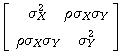 일 때, Y|x ~N(μY +ρ(σY /σX)(x-μX),σ2Y
(1-ρ2)).
일 때, Y|x ~N(μY +ρ(σY /σX)(x-μX),σ2Y
(1-ρ2)).
- Marginal normality does not imply joint normality. (cf.
Exercise 4.47)
4.6 Multivariate Distributions
- 두 확률변수에 관한 성질을 n개의 확률변수에 관한 성질로
확장 (정리 4.6.6, 4.6.7, 4.6.11, 4.6.12)
- Multinomial distribution:
- If (X1, X2,
... ,Xm)~Multinomial(n,p=(p1,p2,....,pm)), where X1+X2+
... +Xm=n, p1+p2+ ...+pm=1,
then Xi ~ b(n,pi)
- If (X1, X2,
... ,Xm)~Multinomial(n,p), then (X2, ... ,Xm)|X1~Multinomial(n-X1, p=(p2/(1-p1),p3/(1-p1),....,pm/(1-p1)))
- [Q] What is the conditional distribution of (X3, ... ,Xm) given (X1,X2)?
- mutual independence와 pairwise independence의 관계 (참고:[Q]
mutually independent sets와 mutually exclusive(or disjoint) sets의 구별;
Definition 1.1.5, Exercise 1.39 참조)
- Example 4.6.13: distributions of order statistics of
exponential distribution and the spacings;
- Let X1, X2,
... ,Xn be a
random sample from Exponential(λ), and Y1, Y2,
... ,Yn be the
order statistics. Then the normalized spacings nY1, (n-1)(Y2-Y1), ..., 2(Yn-1-Yn-2),
Yn-Yn-1 are iid Exponential(λ).
[Q] give a proof of this.
4.7 & 3.6 Inequalities and Identities
- Hölder's inequality: Cauchy-Schwarz inequality and
Liapounov's inequality are special cases. Also see (4.7.9).
- Minkowski's inequality
- Jensen's inequality
- covariance inequality (Theorem 4.7.9)
- Chebyshev's inequality p.122 and Markov's inequality
in p.136 ([Q] What's the difference? [Q] give a proof of Markov's inequality.)
- Example 3.6.2: P(|X-μ|≥tσ) ≤ 1/t2. 이 부등식은 기대값과 분산이 존재하는 모든 확률변수에 적용할
수 있다는 장점이 있으나 너무 무딘(상한값 1/t2이 너무 큰) 단점도 있다. Example 3.6.3과 136쪽 Theorem 3.8.2 참조.
- 3.6절: recursion relations
- Stein's Lemma (Lemma 3.6.5): [Q] What's the use of this
lemma?
제4장 (3.6절) 연습문제(숙제)
5 6 7 11 12 13 14
15 17 19 21 24 26 27 28
31 32 36 39 41 45 47
52 53 54 55 56 58 64 3.44 3.46 3.49(b)